Two 3-d cyclic integrals by Mathematica

This post is converted to Markdown from this Mathematica notebook thanks to the M2MD package by Kuba Podkalicki.

I came across in a paper Counting triangles in power-law uniform random graphs by Pu Gao, Remco van der Hofstad, Angus Southwell, Clara Stegehuis on ArXiv today. Then I spotted two integrals, equation (2.1) and (2.2). These two are left as unevaluated integrals. But they don’t look too intimidating so I gave them a try and voila they have closed form as below:

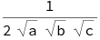
for \(2\leq t\leq 3\).

There is probably a book somewhere that has these formulas. But here I will show you how to use Mathematica to get them.

The first integral

The first one is actually quite easy. You can do it with directly in Mathematica 12.1 without any effort. Let

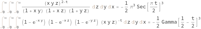
int = Inactive[Integrate][(x*y*z)^(2 - t)/((1 + x*y)*(1 + y*z)*
          (1 + x*z)), {x, 0, Infinity}, {y, 0, Infinity}, 
     {z, 0, Infinity}]

With the assumption

assume = 2 < t < 3;

we can compute this integral symbolically

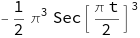
intSym = Assuming[assume, int // Activate // FullSimplify]

To be sure let’s do some numeric verification.

intN = int /. {Integrate -> NIntegrate}

Table[1 - intN/intSym // Activate // Quiet, {t, 2, 11/4, 1/4}]

(*{-9.28939*10^-10, 5.05751*10^-8, 1.48692*10^-7, 0.000287941}*)

As, you can see the relative differences between numeric and symbolic integral are quite small. This increases our confidence that we got the right answer.

The second integral

Let

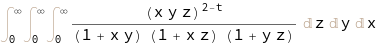
f[x_, y_, 
  z_] := (x y z)^-t (1 - E^(-x y)) (1 - E^(-z y)) (1 - E^(-z x))

We want to compute

int2[1] = Inactive[Integrate][f[x, y, z], {x, 0, Infinity}, 
     {y, 0, Infinity}, {z, 0, Infinity}]

Mathematica cannot do this directly. But we can do a change of variable by integrating \(f(g(a,b,c))\) with

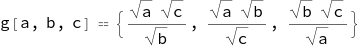
g[a_, b_, c_] := {(Sqrt[a]*Sqrt[c])/Sqrt[b], 
     (Sqrt[a]*Sqrt[b])/Sqrt[c], (Sqrt[b]*Sqrt[c])/Sqrt[a]}

In other words

HoldForm[g[a, b, c]] == g[a, b, c]

We can use the chain rule. First let’s get the Jacobian.

jacob = D[g[a, b, c], {{a, b, c}}] // Simplify // Det

So we can instead integrate.

int2[2] = 
 int2[1] /. f[x, y, z] -> (f @@ g[a, b, c])*jacob /. {x -> a, y -> b, 
   z -> c}

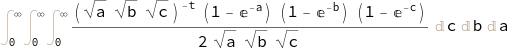
This Mathematica knows how to do

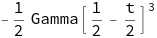
int2Sym = Assuming[assume, int2[2] // Activate // FullSimplify]

Again let’s check numerically. This time it’s a bit bit challenging and you have to play a bit with the strategy of the integration.

Before change of variable.

int2N[1] = Inactive[NIntegrate][f[x, y, z], {x, 0, Infinity}, 
      {y, 0, Infinity}, {z, 0, Infinity}]

After change of variable.

int2N[2] = Inactive[NIntegrate][f @@ g[a, b, c]*jacob, 
      {a, 0, Infinity}, {b, 0, Infinity}, {c, 0, Infinity}]

The differences comparing to the closed form are

Table[1 - {int2N[1], int2N[2]}/int2Sym /. t -> 2 // Activate // 
  Quiet, {t, 2, 11/4, 1/4}]

(*{{1.20381*10^-7, 2.77161*10^-8}, {2.35678*10^-6, 
  2.21698*10^-6}, {0.000204701, 0.000260132}, {0.0251801, 0.0283442}}*)

So again, we can be quite sure that we got the right answer.

Reference

Gao, P., van der Hofstad, R., Southwell, A., & Stegehuis, C.(2018).Counting triangles in power -- law uniform random graphs. ArXiv:1812.04289 [Math].